Maintaining Sharp Features in Surface Construction for Volumetric Objects

 

Eddy Loke and Erik Jansen

 

Discretized Marching Cubes (DMC) is a standard method in computer graphics for constructing 3D surfaces in data represented on a regular grid. After thresholding, it builds high-resolution surfaces by tiling surface patches halfway between the objects and the background. We show that by performing the triangulation at sub-grid level, we can extend the shape domain of the DMC method and maintain concave and convex object features. This makes lower approximation errors and lower triangle counts possible.

 

Keywords: discrete topology, discrete surfaces, boundary triangulation, Marching Cubes, convexity, concavity

 

1.            Introduction

Volumetric models are defined on a regular data grid and can either be rendered with direct volume rendering techniques or with fast polygon rendering hardware. The latter only after extracting a surface model from the voxel data by surface construction algorithms like Marching Cubes [LC87]. To reduce the number of degenerated triangles and to make it easier to merge smaller triangles into larger surface patches, the Discrete Marching Cubes (DMC) algorithm [MSS94] fixes the position of the nodes of the triangulation to the midpoints of the cell edges. This reduces the number of orientations of the triangles to a limited set of discrete orientations, which facilitates merging the triangles into larger surface patches. MC and DMC methods were originally designed for extracting and visualizing isosurfaces for gray shaded data, but they can also be advantageously used for (segmented, thresholded) binary voxel data. As they generate a surface in between the object and the background, they always create a manifold surface, also for isolated points, lines and thin planes. By constructing surfaces at a spatial resolution that is higher than the spatial resolution of the original voxel data we have room to build a manifold surface. Although DMC generates manifold surfaces and optimizes the triangle output, it still has one drawback: it creates oblique surfaces at object slopes but also at sharp edges and corners.

 

In this paper we show that the standard surface mapping by DMC can be derived from a simpler triangulation scheme applied to the eight sub-cells of each cell. By locally adapting the triangulation we can extend the DMC shape domain and preserve sharp features such as convex and concave edges and corners.

 

The structure of the paper is as follows. First we discuss in section 2 surface generation methods on discrete grids, i.e. methods that construct surfaces through the boundary voxels of a volumetric object (see fig. 1). In section 3 we introduce a new triangulation scheme for discrete objects and we apply this scheme to surface methods that generate a surface inbetween object and background such as MC and DMC. We will show how we can reconstruct the standard DMC configurations by first subdividing the cell in eight subcells, and then applying the new triangulation scheme to each subcell. The resulting surfaces are topologically equivalent to those generated by DMC. In Section 4 we show that, if we have a priori knowledge about concave and convex features (edges and corners), we can locally modify the sub-grid and apply a mix of different triangulation schemes to preserve those features. The paper concludes with results in Section 5 and a discussion in Section 6.

 

 

 

 

Figure 1. Object with 6-connected surface (left) and 18/26 connected surface (right)

2.            Discrete surface representations

A volumetric representation consists of a three-dimensional grid of voxel positions, where each voxel position stores one or multiple values. We limit the discussion here to regular grids that constitute a discrete space with points that are either black (the object) or white (the background). Each point has a 3x3x3 neighborhood which are 26-adjacent to the central point[1]. This neighborhood can be decomposed into eight cells (of 2x2x2 voxels). See fig. 2.

 

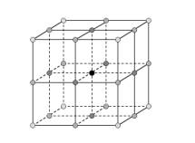
Figure 2. Adjacency relations

 

Since the early seventies, quite some mathematical ingenuity has been invested in the study of boundary voxel configurations to find out under which conditions such a "discrete surface" (consisting of neighboring boundary voxels) has similar topological properties as a regular manifold surface model, i.e. separates correctly the interior component from the exterior component. This is relevant for a large number of operations such as thinning and skeletization, ray casting and boundary construction. The study of these properties is known as digital topology [KR89] and has resulted in several topological sound boundary definitions [MR81], [MB99], [Kov89], [CB99].

 

Couprie and Bertrand [CB99] introduced the notion of simplicity surface, which constitutes a boundary consisting of boundary points that are adjacent and are not simple points. Simple points are points that can be removed from the boundary without altering the topology. Couprie and Bertrand give several operational definitions for simple points and they prove that a simplicity surface can be built out of only eight different 2x2x2 voxel configurations [CB99]. On basis of these configurations it is easy to define a triangulation method for the discrete surface[2].

 

However, the definition of simplicity surface is only of limited value from a practical point of view, as can be seen from the 2D example of figure 3. The black points constitute a discrete object with only one interior point (marked grey) and eight boundary points. If we define the boundary as a 4-connected (analoguous to the 6-connectivity in 3D) chain of points then we have eight boundary points. If we include also the 8-adjacency (the 2D analog of the 18 and 26-adjacency in 3D) then the corner points become "simple", i.e. they do not longer border directly to the interior but only to the outside background.

 

 

Figure 3. 2D example of 4- and 8-boundary

 

In the 3D example of figure 4 (background not shown), the 18/26-surface would be only the octahedron around the interior point (fig. 4b), while the 6-surface would be the full cube (fig. 4a). In most practical cases this would be the desired result. Thus if we want to maintain straight corners then we should eliminate the "short cuts". However, if we have an oblique or curved surface then we would like to use the diagonal short cuts of the 18/26-adjacency to avoid the staircasing of the 6-surface representation (compare fig. 1b with fig. 1a).

 

 

 

Figure 4. 3D example: 6-connected boundary and 26-connected boundary

 

A more practical method was proposed by Kenmochi et al [KII98]. They define the boundary of a discrete object as the outer boundary of the set of discrete simplexes that constitute the object. For 2D, the simplex is a triangle and for 3D a tetrahedron. To construct the boundary, a 3D object is first decomposed into a set of tetrahedra, and after removing the "double" surfaces inbetween the tetrahedra, the single outside faces that are left constitute the overall boundary. The result of this definition is a surface that really encloses the whole object volume and is locally 6-connected in case of convex features such as sharp corners, and 18 and 26-connected in case of obligue surfaces. They also give a cell-by-cell construction method that directly generates a correct surface using 14 possible triangulation configurations for 2x2x2 cells (fig. 5).

 

 

 

 

Figure 5. Kenmochi configurations [KII98]

 

The Kenmochi method is a sound and useful method. It encloses all volume elements inbetween the grid points. However, in some cases the space between boundary points may arbitrarily be assigned to the object or to the background. For instance in cell-configuration P6b, the middle tetrahedron can be arbitrarily assigned to the object or to the background. If the central tetrahedron is removed we get another triangulation (compare fig. 6c with fig. 6a).

 

 

 

Figure 6. Middle tetrahedron in configuration P6b is either included (a) or excluded (c) of the object

 

In these cases the Kenmochi method chooses for the object and not for the background. The method thus generates a surface with a maximum envelop which may not in all cases be the desired result. Further we may observe that convex sharp corners and edges are now maintained, but that the method still generates oblique faces in concave situations due to the fact that the method generates tetrahedra "in the corner" (cf. configuration P6a of fig. 5). If we want to avoid this we should give the background a higher priority than the object, and avoid the "short cut" of the 26-and 18-connectivity, and reduce it to 6-connectivity. However, then we also turn correctly interpolated oblique faces (see fig. 1b) into stair cases, and it would be equal to having only 6-connectivity (fig. 1a).

In the following we will show that there exists an alternative triangulation that gives priority to the background and we will demonstrate this scheme by using the DMC [MSS94] configurations as example.

3.            Background priority method

The Marching Cubes algorithm [LC87] generates a surface triangulation for an iso-surface at the iso-value positions inbetween the grid points of the 3D data volume. Discrete Marching Cubes method (DMC) was presented by Montani et al. [MSS94] as a method to reduce the number of pathological cases in the standard Marching Cubes algorithm. Instead of taking the exact intersection of the isosurface with the edge between neighboring voxels they take the midpoint. This increases the number of 14 MC cell-vertex configurations to 16 cell-vertex configurations for the DMC method. We are in particular interested in their configuration "e", "k", "l", "n", "o" and "p" (see fig. 7).

 

Figure 7. Six of the 16 DMC configurations (cf. Figure 3 in [MSS94]).

 

How the 16 DMC configurations were derived is not clear from [MSS94], but we may assume that they have started with defining a pattern for the faces of the cell (see fig. 8a, b, c and d), and linking the edges of these separate faces and connecting them with the centre point to fan out a 3D triangulation pattern.

 

 

Figure 8. The DMC configurations can be derived from the above 2D patterns. It is arbitrary whether configuration "c" (background priority) is chosen or "e" (object priority).

 

We note that the authors of the DMC method have given priority to the background instead of the object, otherwise the configurations would have been based on the side-configuration "e" instead of "c" (fig. 8). The choice of whether the midpoint (in the DMC configurations) is part of the object is also arbitrary. For instance for the DMC-e configuration it is five white corner points against three black, so it would be more natural to have the center point white, but having the center point black generates a smooth triangulation.

 

An alternative method to construct the DMC configurations is to built them by triangulating the DMC subcells. We first subdivide the cell into eight subcells and then map the 2x2x2 DMC voxel configuration to the new 3x3x3 voxel setting. In the 3x3x3 setting we assign the midpoints the "object/background" classification of the DMC configurations, and then, instead of applying the DMC triangulation directly, we apply the configurations of the Kenmochi method (fig. 5) to the eight individual 2x2x2 cells, with the result shown in fig. 9. We may notice some differences with fig. 7.

 

 

 

 

Figure 9. The DMC configurations derived with the Kenmochi method.

 

In fact, the differences between fig. 6 and fig. 8 are due to the fact that the Kenmochi scheme gives priority to the object while the DMC scheme gives priority to the background (cf. fig. 8c).

 

Looking at the above examples we may wonder whether there exists a triangulation that directly generates the standard DMC configurations. This is indeed so [LJdB06] (see fig. 10). Instead of the object priority (cf. fig. 8e) we follow the DMC convention (cf. fig. 8c) and give priority to the white diagonals. This means that only object voxels are connected that are 6-adjacent. Some of the Kenmochi configurations remain (P3a, P4a, P4e, P6a and P7a), while other configurations reduce to triangles only or to combinations with dangling voxels. P4g has no triangle anymore, only isolated points.

 

 

 

 

Figure 10. Background priority scheme [LJdB06]

 

Now we can built the standard DMC configurations. See fig. 11.

 

 

Figure 11. The DMC configurations with Background Priority algorithm.

 

From these examples we see that the DMC configurations can be built from the 3x3x3 subgrid with the restriction that the cell edges are only black-black, white-white, black-white or white-black voxel combinations (which is due to the 2x2x2 starting situation) and not white-black-white or black-white-black (which would be possible in a free chosen 3x3x3 configuration). There are still some minor differences, due to the triangulation from the centre point in the DMC configurations. Compare for instance DMC-p in fig. 6 and fig. 11.

 

The DMC method implements (6,18)-connectivity, 6-connectivity for the object and 18-connectivity for the background. A (18,6)-connectivity model (e.g. the object priority method) would connect the two 6-connected components which are 18-adjacent in configuration DMC-l and DMC-n, and thus would create non-manifold situations. The (6,18)-connectivity and the absence of white-black-white and black-white-black edges guarantees that no non-manifold situations can occur (e.g. P6b with folding edge does not occur in DMC). Note that the (6,18)-connectivity for the object and background components as such does not seem to imply that we have to limit the triangulation also to 6-connectivity (as is suggested in [KII98]). So it seems useful to discern between object (node) connectivity and surface connectivity.

 

The Background Priority scheme gives a better triangulation for concave features while the Object Priority scheme better serves the convex features (compare fig. 12a with fig. 12b). The two schemes nicely complement each other. Although the two schemes differ in object connectivity, we can easily combine both schemes because there is never a discontinuity between two neighboring cells. The neighboring faces always correctly share the same object and background topology, as can easily be verified from fig. 5 and 9. Only the "folding" edge of P6b in both schemes is not matched by edges in the other topology, which is correct.

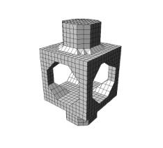
Figure 12. Object priority (left), background priority (right).

 

 

4.            Preserving convex and concave features

In the DMC-method the sub-grid is implicitly used but never explicitly generated. In the following we will present an algorithm to explicitly generate the sub-grid subdivision. By performing the triangulation on each individual subcell, we can locally adapt the triangulation (foreground versus background) in order to preserve sharp features at convex edges and corners. We will also present algorithms to locally extend the subgrid object nodes to better maintain convex features (edges and corners) and we will introduce an enhanced version of the background priority triangulation to represent concave features.

 

To create a classified sub-grid we first subdivide each 2x2x2 cell grid in a sub-grid of size 3x3x3. We keep the classification (black or white) of the corner points but we have to re-classify the new midpoints. We do this by applying the following rules in three passes:

- in the first pass we set any node with two black 6-neighbors to black, this will set edge midpoints between two black corner points to black

- in the second pass we set any node with three black 18-neighbors to black; this will set face-midpoints with three neighboring black corner points to black

- in the third pass we set any white node with a 6-connected black neighbor to black.

Figure 12 exemplifies the sub-grid construction for the DMC-p configuration.

 

 

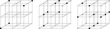
Figure 13. Subgrid construction for DMC-p configuration. Classification of original nodes (left), black nodes added after the first two passes (middle), black nodes added in last pass (right). The black nodes of the last pass carry the surface, the gray ones are internal object points (compare with DMC-p in fig. 11).

 

The first rule guarantees that two black 6-neighbors remain connected via the shortest 6-path. Rule 2 guarantees that two 18-neighbors remain connected via the shortest 18-path. In order to maintain the (6,18) topology, rule 2 can only be applied when the 18-neighbors have a 6-neighbor in common, because two 18 or 26-adjacent components as such may not be connected. The last pass moves the object boundary to the new intermediate points inbetween the original object and the background. If we then apply the triangulation to these new boundary points, then we effectively create a boundary surface inbetween the original object and the background nodes.

 

None of these operations alter the object topology. However, rule 3 always causes a rounded representation of objects, also for objects which originally have sharp edges and corners (see fig. 14a). The surface is biased to the object because rule 3 only extrapolates to nodes which are 6-adjacent to the object (and never to 18- or 26-adjacent directions). In standard situations this is correct but at convex and concave edges and vertices we may want to move the triangulation more "outward" or "inward" to maintain sharp features (see fig. 14b).

 

 

 

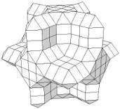
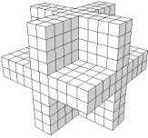
Figure 14. Object without feature detection and BP-triangulation (left) and with feature detection and a mix of triangulation schemes (right).

 

 

For discrete objects there is not a clear definition of "object edge" and "object corner point". There may be regular rows of black nodes that form an convex or concave edge or several rows that culminate into a sharp corner point. In [LJ07] we give some filters to detect regular object features. Of course any definition for "regularity" is arbitrary and can be adapted for the application at hand. Figure 15 gives an example of convex and concave features.

 

 

 

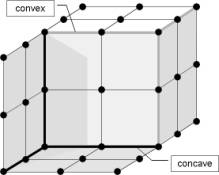
Figure 15. Convex (grey) and concave (black) features (shadow to disambigue figure)

 

The feature detection is done on the original resolution (not on the subgrid). We label the associated nodes as "convex" or "concave". Note that each node may have different labels for different directions. We can maintain convex features in the subgrid by adding extra object nodes (i.e. extraploate and interpolate the subgrid). For convex edge feature points we set the 18-connected white nodes to black and for convex corners the 26-connected white node, and label them with the "convex" label. For the concave features we do not need to add extra black nodes, we only pass the "concave" label to the nearest 18/26 connected white nodes.

 

Next we have to guarantee that the triangulation goes through the classified feature points. For the convex cases this is simple, i.e. it suffices to apply the OP-scheme because this triangulation scheme encloses all object nodes. For the concave case, however, we have to explicitly force the surface through the concave feature points. For instance, in figure 13b the triangulation is adapted to the concave feature points.

 

For most cases, this can be achieved with a 6-connected triangulation. However, the 6-connected triangulation does not always suffice. For instance for P7a (see fig. 16), the concave feature point(s) can only be included in the surface by "pulling" the triangulation to the feature point(s). We call these variants "strong-background-priority". The cell with P6b in the centre of fig. 14a is turned into the configuration bottom-right of fig. 16 in fig. 14b.

 

 

 

 

 

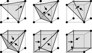
Figure 16. Triangulation of P6b (top-left) and some of the triangulations for one, two, three and four concave feature points (marked grey).

 

Note that for some cases the connecting triangle removed. This means that for cells that share a feature point, the same procedure has to be applied to maintain consistency in the connection. In [LJ07] we give the full LUT for all possible feature point classifications and corresponding triangulations.

5.            Results

Figures 17 and 18 show the surfaces generated by detecting the different types of edges and corners for various objects.

 

 

 

 

 

 

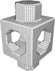
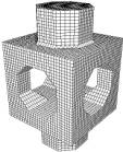
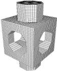
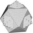
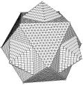
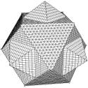
Figure 17. Hoppe figure (top) and dice (below), from left to right: standard DMC, feature-enhanced grid and BP, feature-enhanced BP+OP, feature-enhanced BP+OP+strong-BP.

 

 

 

 

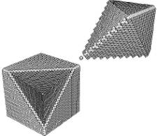
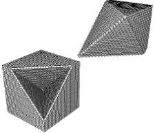
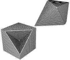
Figure 18: Standard DMC-surface (top-left), with convex edges and corners with BP (top-right); with OP for convex diagonal edges and corners (bottom-left); with strong-BP for concave corner (bottom-right)

 

6.            Discussion

We have shown that we can simulate DMC triangulation by creating a subgrid, classifying the new nodes, and applying a background priority surface model to the individual subcells. Further we have shown how we can preserve convex and concave features, using a mix of OP and BP schemes. The advantage of working in DMC sub-space is that there is room to build surfaces (oblique or sharp) which are guaranteed to be manifold for any input data.

 

In our apprach the feature detection is not done on the resulting triangulation which would normally be the procedure (e.g. [KBSS01]) but we detect features directly on the original volume data, after segmentation but before triangulation. Nowadays, excellent discrete feature detection algorithms are available for binary data, but also for grayvalue data [LLZ01].

 

Discrete algorithms are normally faster than algorithms which are applied in continuous space. For future research we will look at application of the framework for isosurfacing grayvalue data. Interpolated isosurfaces can be built first by positioning nodes in DMC sub-space, and then, depending on the grayvalues move them along the straight trajectory between the nodes to the position that corresponds with the exact iso-value, without losing the guarantee of surface manifoldness and with the a priori features already in place.