Acquisition and Rendering of Paintings [1]

 

Ewald Snel, Jurriaan Heuberger, Wouter Pasman, Erik Jansen

 

For interactive visualization of paintings on a computer screen, a framework is presented that offers practical methods for image-based acquisition, compression, and rendering of paintings. The aim of the framework is to create digital reconstructions of paintings that offer all the view point dependent reflection properties of the real paintings.

The 3D reflection characteristics are described by a mathematical model based on the Lafortune reflection model. The parameters for this model are determined from a set of pictures of the painting taken under regulated light conditions and viewing angles. For describing surface structure, the reflection model was extended with support for normal vectors. In addition, the surface height was recovered for accurate alignment of surface structure in the images. After correction and alignment, the reflection model is fitted to the image data and then implemented on the graphics card of a standard PC. The painting can then be viewed in realtime under different viewing directions and lighting situations, showing all the directional reflection properties of the real painting.

1.            Introduction

Almost every piece of art in the world is now visually accessible through the web in the form of digital photos. Although these photos may be taken carefully, they can never convey the same spatial impression as observing the real piece of art. A still image only records the reflection for one single viewing position. To get a convincing 3D impression we should see the changes in reflection as we move our head.

 

We can simulate this by using the latest graphics hardware and so-called image-based rendering techniques. Image-based rendering uses photographs of the real object to synthetically reconstruct the shape and reflection of the object. With this reconstructed information, high-quality synthetic images of the object can be rendered in realtime and from any chosen view position and within any chosen lighting environmentMcA02.

 

 

 

 

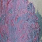
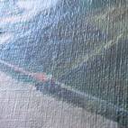
Figure 1. Specular reflections provide insight into the surface structure of the painting, visualizing paint blobs (left) and canvas (right).

 

The reflection behavior of a surface such as a painting is in fact a complex phenomena. The reflection is partly based on the physical properties of the surface and partly a result of the geometric surface details. The physically-based reflection component is generally represented by a Bidirectional Reflection Distribution Function (BRDF), which describes the amount of scattering, dispersion and absorption of the incoming light. If the reflection is only local than the BRDF is a 4D function that describes how incoming light from all directions is reflected into all outgoing directions. When we also consider sub-surface scattering - as will occur in a painting with a lacquer layer - then the function is even more complex. Further, the BRDF may change over the surface because of local differences in the chemical composition and colour of the paint. This spatial BRDF version is often denoted as SBRDF or as Bidirectional Texture Function (BTF)Da99.

 

In standard computer graphics the BRDF is most of the times simplified to a simpler reflection model (Phong-model) with a uniformly spread diffuse part and a specular "lobe" that represents the direction-dependent mirroring reflection. In this work we will apply the more sophisticated Lafortune modelLaf97 that uses multiple lobes for both the specular and diffuse reflection, with extra parameters to describe retro-reflection, off-specular peaks and increasing or decreasing reflectance at grazing angles. (see Figure 2). An earlier master thesis project by Jurriaan Heuberger indicated the suitability of the Lafortune reflection model for describing the reflection properties of paintingsHeu05.

 

 

 

(to be added)

 

 

Figure 2 Phong (left) and Lafortune (right) reflection model

 

Next to the material properties, also surface geometry contributes to the amount of light scattering. Deviations from perfect flatness are generally categorized into three levels, macro-geometry, meso-geomemetry and micro-geometry. Micro-geometry represents high-frequency variations, corresponding to small surface details such as surface roughness and orientation of small geometric patterns (grooves). It is not easy to measure these variations in detail, so they are normally included in the BRDF. Meso-geometry corresponds with medium sized surface variations such as small ridges and protusions, such as from the canvas pattern and paint blobs (see Figure 1). To a certain extent we can measure these local depth changes using different views of the surface.

Finally, macro-geometry refers to the three-dimensional shape of the object. As a painting is normally flat, we will ignore the macro geometry and render the painting as a flat polygon with texture mapping to model the local depth changes (depth mapping), the orientation of the surface (normal mapping), and the BRDF changes (parameter mapping).

 

In this project we have followed to a great extent the approach of McAllisterMcA02. A test painting was photographed from different viewing positions and under different lighting conditions, and from these images for every point on the surface of the painting a BRDF was reconstructed. After mapping the SBRDF to the graphics hardware we were able to render the painting in realtime from any viewpoint and under any lighting condition. For this project a special painting was created by Jurriaan Heuberger that shows different patches of paint with one or multiple layers of farnishHeu05. The real and synthetic result are displayed in Figure 3.

 

 

	Original photo		Computer reproduction

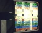
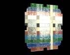
Figure 3. Photograph of painting (left) and computer simulation (right).

For a video demo see http://graphics.tudelft.nl/student_projects/heuberger/

 

The whole procedure has the following steps:

·       acquisition of the painting by taking a few hunderd pictures from well chosen view points and light source positions (section 2)

·       alignment and registration of the images into a rectilinear format, such that all image data for each location of the painting (each pixel) is grouped together; this rectification compensates various spatial distortions such as lens distortion of the digital camera, perspective distortion caused by taking pictures under various view angles and distortion caused by the surface structure of the painting (section 3).

·       correction for differences in lighting at different points on the surface, and for colour distortions due to overexposure (section 4)

·       fitting of the mathematical model to the reflection data for each pixel (also section 4)

·       implementation of the reflection model on the graphics hardware by a decomposition into 2D functions and rendering of the model with an environment map for providing a realistic lighting environment (section 5).

 

 

2.            Acquisition

 

For the acquisition the following setup was built (see Figure 4)

 

 

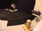
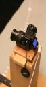
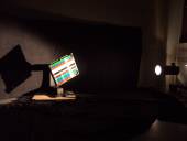
Figure 4 Overview of the measurement setup.

A computer-controlled digital camera was mounted on a trolley that could rotate around the painting (Figure 4 left). The painting was mounted on a frame with a ball joint that could be rotated in any direction. The lamp was positioned at discrete positions in a horizontal plane. The painting was further stiffened with a wooden frame to avoid changes in the bending of the painting during measurements.

Figure 5 illustrates how a triplet of rotations of the spherical joint and the angle of rotation of the camera in the horizontal plane can simulate the position of the camera and light source, relative to the painting, in the left image.

 

 

 

 

 

 

 

 

 

Figure 5 Desired model of camera and lamp position relative to the position of the painting (left) and the actual setting using a spherical joint for the painting and moving the camera in a horizontal plane (right).

 

 

 

 

 

 

 

 

 

 

 

 

 

 

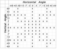
Figure 6 Positions of the camera, relative to the specular mirror direction.

 

Most of the variations will occur near the specular highlight. So to make optimal use of the photos, a sampling pattern was chosen that concentrates the sampling around the direction of the specular highlight and less in other directions (see Figure 6)Heu05. In addition, support for anisotropic reflections was dropped to limit the primary measurement set to 690 samples, with an additional 80 samples for accurate determination of surface normals.

 

A few of these samples are shown in Figure 7.

 

Figure 7 Samples 100-105, gamma and white balance corrected for illustration

To avoid variations in the light intensity of the lamp, a stabilized 12 V DC power supply was used with an additional 220V DC/AC power inverter. Measurements indicated that the light output of the lamp, after an initial warming up period of about 15 minutes, was nearly constant. There was some noise left on the blue channel, which might be related to the relatively low sensitivity of the camera's CCD sensor to blue colors.

 

3.            Alignment and rectification

The result of the acquisition, as described in section 2 is a series of photographs of the painting under various angles. Corresponding points at the painting, however, do not appear at the same pixel position in the images. In order to have all reflection data available for each point, the images need to be re-aligned such that all aligned images resemble an orthogonal frontal view of the painting and each pixel on each of the corrected images roughly corresponds to the same part of the painting.

 

The alignment process consists of three steps:

Lens distortion

Zoom lenses often exhibit some degree of radial distortion, depending on the design and quality of the lens system and the zoom factor used to take the photograph. These distortions can easily be corrected using a 5^th order polynomial approximation. This correction can be derived by photographing a test image and measuring the barrel distortion. This is the first step in aligning the images and is applied to the raw photographs.

Perspective correction

The perspective correction step compensates for any rotation or translation of the painting relative to the camera. To measure the perspective distortion, markers were attached to the corners of the frame where the painting was attached to. The markers could have been detected automatically in the image but for some of the viewing angles the marker detection was not good enough and an interactive interface was developed to select the exact marker position.

 

Figure 8 Transformation tool, showing marker selection (left view) and aligned result (right view).

 

From the retrieved marker positions the parameters for perspective correction can be estimated. In combination with a zoom factor, this produces a projection matrix for warping the image to a frontal view of the painting. This step is also known as rectification, because of the rectangular images it creates.

 

 

Depth correction
The applied BRDF model is not suitable to capture meso-geometry information. Therefore, an additional depth correction step is used to compensate for surface relief. The depth correction is applied to the images to improve the alignment, but the same information will later be re-used in the display to bring back the relief into the synthetic picture. This will be done with displacement mapping, which is a technique to simulate local depth variations on a flat surface.

 

 

 

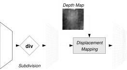
Figure 9 Displacement mapping, which uses the depth map to generate relief on a flat surface.

 

The actual depth changes over the painting are measured using a mesh that tiles the image. The graphics interface for setting the perspective correction was extended with the option to visually overlay two different views of the painting. By manually adapting the position of the individual nodes of the depth mesh and applying the derived depth correction to the two images, the depth values can be manually adjusted until the two image completely overlap. Any change to the depth will immediately appear as improvement or worsening of the alignment of corresponding parts of the painting (see Figure 10).

 

 

Figure 10 Figure 24: Displacement of about 2 pixels for samples 10F1s.tif (left) and 30A5s.tif (right).

 

Since some parts of the painting lack easily distinguishable features that can be used for alignment, the depth map can be less detailed in such areas. For that reason, the editor has a user selectable subdivision level that determines the scale of changes made to the depth map. At the highest level, the editor operates on a single depth map value, whereas lower levels operate on a smaller tile of the image. When editing at lower subdivision levels, changes are cubic interpolated over the entire region and written to the depth map. Figure 11 shows the depth map constructed for the painting.

 

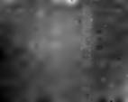
Figure 11 Depth map for the painting. Black to white values correspond with a distance of -1.49 to 2.44 mm

For each image tile (of the depth map), a transformation matrix is calculated that warps the raw photograph to a correctly aligned image. This warping transformation includes the global correction for lens distortion, the global perspective correction and the local depth correction. The warping is implemented on the pixel/fragment shaders of the graphics card using the texture mapping facilities of the graphics hardware. The separate rendered tiles are finally merged into one correctly aligned image. This process is done for all pictures.

 

4.            Fitting

The fitting process takes the measured values for each pixel and adjust the parameters of the Lafortune model such that the lobes correctly describe the measured data with some approximation and smoothing. This adjustment is done with several iterations using the standard Levenberg-Marquardt algorithm Lou05.

 

To better represent some of the meso-geometry effects, the Lafortune reflection model has been extended with support for arbitrary normal vectors. These normal vectors can compensate for changes in surface orientation, caused by brush strokes, paint blobs and canvas structure. The surface orientation is calculated during the fitting and is used later as well for the display, greatly enhancing the depth impression of the resulting picture (see Figure 12).

 

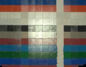
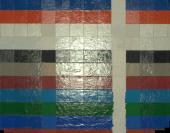
Figure 12 Result of the rendering without (left) and with normal correction (right)

 

Before we can actually do the fitting, some additional corrections have to be done to compensate for differences in the incoming light and for correcting overexposed samples. The correction for differences of the incoming light for different points of the painting is relatively easy as the received light intensity is a function of the cosinus of the angle between surface and direction of the incoming light, and decreases quadraticly with the distance between the light source and the illuminated object. Compensation for overexposure is more involved.

Compensation for exposure

Reflectance data generally has a high dynamic range. This is mainly caused by highly specular materials, where light reflection is concentrated around the mirroring direction. As a result, specular peaks have a much higher light intensity than off-specular reflections. Diffuse materials on the other hand, have a more gradual decay of light intensity away from the mirror direction. The light intensity is also generally much lower than that of specular peaks.

 

Unfortunately, most ordinary digital cameras have a very limited dynamic range, usually represented as linear coded integers. This will either cause diffuse reflections to appear extremely noisy or part of the specular peaks to be overexposed.

The exposure setting of the camera was set as low as possible while not exceeding the maximum allowed noise level for diffuse reflections. However, even at this low exposure setting, some pictures were still partly overexposed. This mainly occurred when taking measurements near the specular mirror direction.

 

CCD sensors of digital cameras convert light intensities into color levels, typically in triplets of red, green and blue. The digital camera used in this experiment has a 8 megapixel CCD sensor, which contains twice as many green as red or blue sensor elements. This ratio of green and red/blue sensor elements is based on the relative sensitivity of the human eye to these primary colors.

 

Reconstruction of overexposed highlights is based on the notion that sensors for different colors vary in sensitivity with respect to the white balance. Considering the mercury lamp has a color temperature of 5500K (nearly white), colour changes are assumed to be mainly caused by the digital camera. Green elements are almost three times more sensitive than blue elements at the same light intensities. Red elements are somewhere in between, being about twice more sensitive than blue elements. As a result, green colors are accurately represented in dark areas, but become saturated in light areas, whereas blue colors appear more noisy in dark areas, but better represent higher light intensities.

 

 

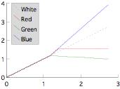
Figure 13 Relative sensitivities for red, green and blue sensor elements.

The relatively low sensitivity of the blue sensor elements results in blueish colors of specular peaks, caused by clamping of the green and red components. Although there is no certainty about the real color of the specular peak, the luminance (the overall light intensity) is assumed to be more accurately described by the unclamped component, in this case the blue. To estimate the chromaticity of the overexposed highlight, one of the other samples (of the same pixel) that is just not overexposed, is taken instead. Then the luminance of the overexposed highlight is reconstructed by scaling the clamped green and red component to meet the chromaticity distribution of the non-overexposed samples.

 

Figure 14 Chromaticity of highlights

The result of this reconstruction is shown in Figure 15. Even though the reconstruction of the highlight is not fully accurate, visual comparison clearly favors this result over the clamped or unclamped original.

 

Original		Clamped to white		Reconstructed

Figure 15 Highlight reconstruction compared to original. The overexposed highlights are left untouched in the original image (left) and are removed in the clamped image (center). The reconstructed image (right) uses the heuristic method described in this section.

The fitting

The succes of the fitting is dependent on several factors:

§       The images should be correctly aligned such that each change in the BRDF happens more or less synchronously for all measured, i.e. all directions at a pixel should behave similarly and not show a different pattern due to lateral displacements of the separate images (for correct meso-geometry we need an alignment accuracy within half pixel ??).

§       The chosen mathematical model should be flexible enough to fit to the distribution of the data points

§       It helps to start with good initial guesses as starting values. We can take these from already processed neighboring pixels or they can be taken from existing databases of exactly measured paint samples.

The fitting is divided into three passes:

§       First, the orientation of the normal vector is determined

§       Secondly, the parameters of the Lafortune model are fitted to the luminance value of the input data

§       Finally, the diffuse and specular colors for the extended Lafortune model are determined.

 

The use of separate passes to fit the luminance and chromaticity components of the reflectance function greatly improves the quality of the fit. Using a third separate pass to fit the normal vector also produced better results then integrating the deviation of the orientation implicitly in the Lafortune reflectance function.

 

The normal vector is estimated by fitting a simplified reflection model to the luminance measurements. The reflection model used for this purpose is a cosine lobe model with a diffuse term and one specular lobe. Fitting of the cosine lobe model is started with a specular lobe with a moderate (soft specular) exponent of 20.0 and the normal vector pointing towards the z-axis. This choice produces accurate results for both specular and diffuse reflections (see Figure 16). Using Levenberg-Marquardt, the parameters are optimized and the specular lobe gradually approximates the input data.

 

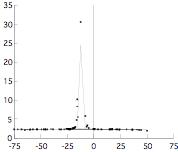
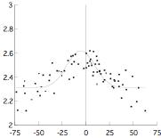
Figure 16 The cosine lobe model can successfully estimate normal vectors for specular (left) and diffuse reflections (right). The gray line indicates the cosine lobe that was fit, its peak indicating the direction of the normal vector. It also works reliable in the presence of noise (see right image).

For diffuse materials, it is not just the specular lobe that determines the direction of the normal vector. The diffuse component can influence the result as well, because the normalization of incoming light depends on the direction of the normal vector. In theory, it is possible to determine the normal vector for completely diffuse materials. However, the accuracy of the normal vector will be much lower, since light intensities vary less with normal direction in such cases than they do for specular reflections. Another aid in estimating the normal vector for diffuse materials is the choice of the exponent for the starting condition. The specular lobe can change to a directional diffuse lobe if necessary, as can be seen in the right image of Figure 16.

 

One of the alternatives tested early in the project was using the peak signal for estimation of the normal vector. Unfortunately, this produced poor results. The cause for this is its sensitivity to noise, because in the end, only one sample is used to compute the normal vector. Another weakness of this method is that the accuracy of the normal vector is limited by the resolution of the sampling pattern. In this case, the smallest step size of the sampling pattern is 3°, which directly determines the maximum accuracy of the normal vector.

 

 

 

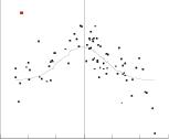
Figure 17 Incorrect normal vector when using peak signal. The red dot indicates the peak signal, the gray line the cosine lobe normal fit.

 

Another option that was briefly investigated was the use of filter kernels to reduce some of the problems of the peak signal approach. Although it did improve the overall result, the choice of the filter kernel was very dependent on the input data. When the filter kernel is too small for the input data, the algorithm is sensitive to noise just as the first method. On the other hand, when the filter kernel is too wide, the results are inaccurate and often erroneously pointing towards the z-axis.

 

The second pass fits the diffuse intensity and specular lobes of the Lafortune model. This pass only operates on luminance values, assuming the shape and size of the lobes is mostly determined by luminance data and much less by color. By splitting up the Lafortune model in a luminance and chromaticity pass, the quality of the fit was greatly improved. Although not described in his paper, McAllister used this procedure for fitting the Lafortune reflectance function in his softwareMcA02.

 

The normal vectors of the first pass are now part of the input data. First the specular lobes are fitted, one more lobe at a time. The starting condition for the first three lobes is a specular lobe with an exponent of 50.0, a directional diffuse lobe with an exponent of 5.0 and a lobe with a moderate exponent of 20.0 respectively. This fitting process is visualized in Figure 18.

 

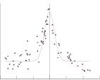
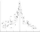
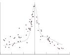
Figure 18 Example of fitting one more lobe at a time, using 1, 2 and 3 lobes from left to right respectively. The black dots are measurements and the gray line visualizes the fitted reflectance function.

This process continues until the maximum number of lobes have been fit or the error criterion starts to increase. There are two advantages to this approach. In the first place, the result of the fit is much better than when all lobes are fit simultaneously. In addition, if the error criterion starts to increase, the fitting process is interrupted and the previous fit is used as the final result. This ensures that the number of lobes used in the end result is optimal with respect to the error criterion, which is sometimes lower than the maximum number of lobes to be tried.

As mentioned earlier, the starting condition is best based on the characteristics of the paint. A varnish layer, if present, produces highly specular reflections, which have the greatest influence on the reflectance function apart from the diffuse term. The paint itself often exhibits more diffuse reflection, best described by a directional diffuse lobe.

 

After the parameters of the Lafortune reflectance function are known, the diffuse and specular albedos can be fit.

5.            Rendering

The final step is the rendering. Because we have extracted the BRDF of the painting we can display the synthetic reproduction of the painting for any viewing position and under any feasible light condition. In normal life light comes from many directions and not from one light source as is often the case in computer graphics. A natural lighting situation can be simulated with an environment map, which is a wide angle photograph of the environment, effectively capturing the incoming light from all directions to the point where the picture is taken. The environment map is stored as a cube map. In this representation, the environment is projected onto the six sides of a cube. Hereby, the environment map can be perceived as a large grid of point light sources, where each pixel in the environment map represents a light source of the pixel's color and light intensity.

The reflection for a point on the surface is calculated by calculating a weighted average of the lobes of the BRDF model with the environment map. This integration takes some time and we can speed this up by moving this calculation to a preprocessing that replaces the environment map with a new version where each direction in the map a value is stored representing the result of a convolution of a lobe with the environment map for that direction. A simple look-up in the map for the reflection direction then directly provides the same answer as the weighted average. For multiple lobes we use multiple environment maps.

 

 

Figure 19 Interface of rendering program

 

For visualizing the painting under different light conditions, the user has the ability to select from a number of different environment maps or supply their own. Different environments result in different reflection effects, as illustrated in Figure 20. The environment maps that were used were created by Paul DebevecDeb

 

 

 

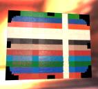
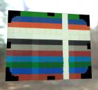
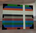
Figure 20 The environment influences the appearance of the painting. From left to right, the painting is visualized inside a church, outside (sunlight) and inside a kitchen. Highlights are more pronounced inside the church (left) with sunlight coming in through the windows only, whereas outside (center) shows more diffuse reflections.

 

For interactivity and realtime display we need a high rendering speed which only can be achieved with use of a graphics card. To be accessible for the fragment shaders of the graphics card, the parameters of the reflectance function need to be stored in a form that can be accessed efficiently by the fragment programs. Taking hardware limitations into account, the most suitable representation are 16 bit integer textures that represent texels as values of [0...1] to fragment programs. These textures can store up to four parameters in one location: red, green, blue and alpha. For efficient texture access, the parameters of the Lafortune reflectance function are paired accordinglyMcA02.

6.            Future work

The resolution of the reconstruction is currently limited by the accuracy of the alignment of the samples, which can be improved considerably. This would also improve fitting of the model, and subsequently, increase the quality of the model as well.

 

A full description of this work can be found in Sne07. The software can be downloaded from http://graphics.tudelft.nl/student_projects/heuberger/

 

References